This is part of a series on a family of dimension-reduction algorithms called non-linear dimension reduction. The goal here is to reduce the dimensions of a dataset (i.e. discard some columns in your data)

In previous posts, I discussed the MDS algorithm and presented some key ideas. In this post, I will describe how those ideas are leveraged in the Isomap algorithm. A clojure implementation based on core.matrix is also included.

Intuition

Isomap uses the same core ideas as the MDS algorithm:

• Obtain a matrix of proximities (distances between points in a dataset).

• This distance matrix is a matrix of inner products.

• An eigendecomposition of this matrix gives us the lower dimension embedding.

Isomap differs from MDS in one vital way - the construction of the distance matrix. In MDS, the distance between two points is just the euclidean distance.

In Isomap, the distances between points are the weight of the shortest path in a point-graph.

The point graph is constructed by placing an edge between two points if the euclidean distance between them falls under a certain threshold or between a point and its top $ k $ neighbors.

This distance matrix captures the underlying manifold more accurately than one constructed using euclidean distances. The following toy example demonstrates this:

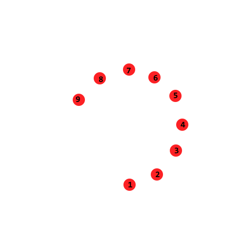
The data shown here looks like a swirl that starts at point 1 and ends at point 9. We would like to recover this phenomenon in our lower-dimension embedding.

The first step is to build a distance matrix. Say we use euclidean distances between two points as the corresponding entry in the distance matrix.

In this figure, it is clear that euclidean_distance(1, 6) = euclidean_distance(1, 8) and euclidean_distance(1, 5) = euclidean_distance(1, 9).

Clearly the distances computed here miss the “swirl” in the data entirely. Working with the point graph mentioned above helps us get around this problem.

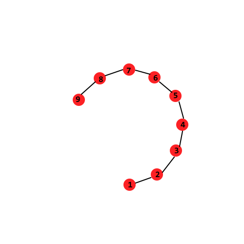
Let us build a point graph by adding an edge between a node and its nearest neighbor (so $ 1-NN $). The weight on the edge is the euclidean distance between the nodes. The distance between two points is the weight of the shortest path between these points. The point graph is shown below:

Observe that when we use this newer distance metric, distance(1, 6) is indeed less than distance(1, 8) and distance(1, 5) is indeed less than distance(1, 9)

This distance function is clearly doing a better job of capturing the “swirl” in the data.

The Isomap algorithm uses a distance matrix constructed like this in place of one constructed with euclidean distances. This distance matrix is then plugged into the MDS framework and an eigendecomposition is run on the double-centered matrix.

Implementation

Let us do a clojure implementation.

We have a point-set as a core.matrix matrix. First, we compute the point-graph. I am going to place edges between a point and its 3 nearest neighbors (so $ 3-NN $). This routines expects a map of the type {point-index point-vector, …}

 1
 2
 3
 4
 5
 6
 7
 8
 9
10
11
12
13
14
15
16
17
18
19
20
21
22
23
24
25

(defn build-point-graph
  "A point graph is a k-NN graph. Edges between
   a point and its 3 nearest neigbors"
  ([indexed-points]
     (build-point-graph indexed-points 3))

  ([indexed-points num-neighbors]
     (reduce
      (fn [acc pt]
        (let [other-points (filter
                            (fn [x]
                              (not= (first x)
                                    (first pt)))
                            indexed-points)]
          (merge
           acc
           {(first pt) (map
                        first
                        (take num-neighbors
                              (sort-by
                               #(distance (first pt)
                                          (first %))
                               other-points)))})))
      {}
      indexed-points)))

Then a simple Floyd Warshall algorithm implementation that computes the weights on the shortest paths. It takes the graph built in the previous step and the original indexed points and builds the graph.

 1
 2
 3
 4
 5
 6
 7
 8
 9
10
11
12
13
14
15
16
17
18
19
20
21
22
23
24
25
26
27
28
29
30
31
32
33
34
35
36
37
38
39
40
41
42
43
44
45
46
47
48
49

(defn floyd-warshall-distance
  "Expected graph representation:
    {V -> neighboring-points}"
  [a-graph indexed-points]
  (let [indexed-points-dict (into {} indexed-points)
        edges    (reduce
                  (fn [acc [x neighbors]]
                    (concat acc (map (fn [n] [x n])
                                     neighbors)))
                  []
                  a-graph)

        inf-matrix (+ Double/POSITIVE_INFINITY
                      (zero-matrix (count indexed-points)
                                   (count indexed-points)))

        zero-diag  (reduce
                    (fn [acc i]
                      (mset acc i i 0))
                    inf-matrix
                    (-> indexed-points count range))

        weights-init (reduce
                      (fn [acc [x y]]
                        (mset acc
                              x
                              y
                              (distance
                               (indexed-points-dict x)
                               (indexed-points-dict y))))
                      zero-diag
                      edges)]

    (reduce
     (fn [old-distances [k i j]]
       (if (< (+ (mget old-distances i k)
                 (mget old-distances k j))
              (mget old-distances i j))
         (mset old-distances
               i
               j
               (+ (mget old-distances i k)
                  (mget old-distances k j)))
         old-distances))
     weights-init
     (for [k (-> indexed-points count range)
           i (-> indexed-points count range)
           j (-> indexed-points count range)]
       [k i j]))))

Once we have a distance matrix, we can simply feed it to MDS:

1
2
3
4
5
6
7

(defn isomap
  "Takes indexed-points and the target dimension"
  [points n]
  (let [indexed-points (map-indexed (fn [i x] [i x]) points)
        graph (build-point-graph indexed-points)
        distances (floyd-warshall-distance graph indexed-points)]
    (mds/distances->points distances n)))

And that’s it!

Examples

I will use word-vectors from word2vec for these 10 words: river lake city town actor doctor dog cat animal home

The word vectors for these words are available in foo.csv.

Let us reduce these to two dimensions. We get:

ISOMAP Embeddings

The embeddings produced by the MDS algorithm are:

MDS Embeddings

Compared to the plot produced by MDS, we have more separation between terms - for instance cat and dog are place close by but they don’t overlap (unlike the MDS plot). This is a qualitative analysis, it is pretty hard to gauge which embedding is better.

Full Source

See this repo: https://github.com/shriphani/clojure-manifold