In the past few blog posts, I covered some details of popular dimension-reduction techniques and showed some common themes. In this post, I will collect all these materials and tie them together.

Dimension?

The best definition I’ve seen for the topic comes from Benoit Mandelbrot’s work on fractal geometry. The fractal dimension is associated with the ability of a pattern to fill space. Here’s a good example to illustrate what we mean.

Consider a curve viewed at three different scales (image stolen from Chris Burges’s document on dimension reduction):

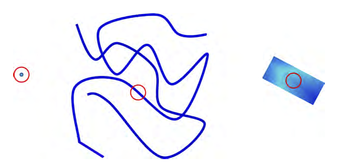
Now, at a microscopic level, we begin observing. How do we observe? Assume that a there’s a sphere around the observer. Now, let this sphere expand a bit. At the microscopic level, your sphere encounters more of the curve’s material in 2 dimensions. This is illustrated in the rightmost figure.

Now, at a slightly different scale, when our sphere expands, we observe more material along just 1 dimension. This is illustrated in the middle figure.

On a scale like the one in the leftmost pic, we encounter no material at all. This is akin to a zero-dimension figure (a point).

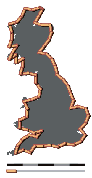
An intuitive explanation of why scale matters is provided in this Wikipedia example. Using a ruler of different lengths, we obtain different measures for the coastline of Great Britain. At various levels of scale, we acquire various measures of the coastline - using a ruler that is as long as the diameter of the earth, the coastline of britain is a negligible fraction of our instrument.

There’s a neat formula that can be used to estimate the fractal dimension of a dataset:

• $ n $: The number of pairs of points in our data.
• $ r $: The radius of a sphere centered around the observer.
• $ p $: The number of pairs of points in a sphere of radius $ r $.

The estimate of the fractal dimension is given by the slope of $ \log(p) $ vs $ \log(r) $.

For the curve in the example above, this value is some real number between 1 and 2 (so the points on the curve have more freedom than those on a line but less freedom than those on a 2D-plane).

A First Stab at Dimension Reduction

Working with intuitions we developed in the first section, we can develop a greedy algorithm:

• Estimate the fractal-dimension of the dataset.
• Choose a dimension (column) to drop, drop it and recompute the fractal-dimension. If the dimension doesn’t change too much (stays within a certain tolerance), consider this dimension dropped.
• Repeat until no more dimensions can be dropped without significantly altering the fractal-dimension.

This is the Grassberger-Procaccia algorithm.

It is intuitive to grasp.

However, in a high-dimension setting, our technique for estimating fractal dimensions falls apart.

In a high-dimensional setting, pairwise distances between the points in a dataset are tightly clustered about a mean. Essentially, the points seem to be equidistant from each other. A Hoeffding bound is provided in this blog post that illustrates this point.

The PCA

One common attempt at reducing dimensions is capturing directions of maximum variance. The PCA projects points in the dataset along the eigenvectors of the covariance matrix. Since this technique is well-known, I’ll just point to this Wikipedia article.

From Proximities to Datasets

A family of techniques I like a lot operate on proximity matrices. A proximity matrix is a symmetric matrix containing similarity scores between the points in a dataset (thus this matrix contains $ n $ rows and $ n $ columns where $ n $ is the number of points in the dataset).

A simple argument demonstrates that proximity matrices are gram matrices (a gram matrix is a close cousin of the covariance matrix). One can retrieve a collection of points for a given gram matrix - see this blog post for a proof.

This family of techniques formulates the dimension-reduction problem as such: “Find a configuration of points in a lower-dimensional place that preserves the proximities in the proximity matrix”.

The standard MDS algorithm uses euclidean distances between points to populate the proximity matrix. This blog post contains more info about this algorithm.

A variant of this algorithm uses path-weights in a $k$-NN graph. This is the Isomap algorithm - covered in this post.

The Kernel Trick

The Kernel trick is leveraged in settings where we transform our points to a higher-dimensional space to make the desired insight pop out. This desired insight is a hyperplane to separate two different classes when working with a classifier. In Kernel PCA, the desired insight is capturing variances so you can run a PCA on the newer dataset in a higher-dimension.

Interestingly, MDS and Isomap are all variants of the Kernel PCA - a topic explored in this blog post.

Up Next

In future blog posts, I will discuss scaling issues with spectral algorithms, insights that can be transferred to other domains and so on.