I just finished rendering the Gridded Population of the World (GPW) dataset. I chose the cyan on black color theme since that is a staple of all my cartography projects. Some insights that people pointed out:

In a previous post, I described the MDS (multidimensional scaling) algorithm. This algorithm operates on a proximity matrix which is a matrix of distances between the points in a dataset. From this matrix, a configuration of points is retrieved in a lower dimension.

The MDS strategy is:

• We have a matrix $ D $ for distances between points in the data. This matrix is symmetric.
• We express distances as dot-products (using a proof from Schonberg). This means that $ D $ is expressed as $ X^T X $. (Observe that $ X^T X $ is a matrix of dot-products).
• Once we have $ X^T X $, dimension reduction is trivial. Running an eigendecomposition on this matrix will produced centered coordinates. The low-dimension embedding is recovered by discarding eigenvalues (eigenvectors).

Thus, assuming that we work with euclidean distances between points, we retrieve an embedding that PCA itself would produce. Thus, MDS with euclidean distances is identical to PCA.

Then what exactly is the value of running MDS on a dataset?

First, the PCA is not the most powerful approach. For certain datasets, euclidean distances do not capture the shape of the underlying manifold. Running the steps of the MDS on a different distance matrix (at least one that doesn’t contain euclidean distances) can lead to better results - a technique that the Isomap algorithm exploits.

Second, the PCA requires a vector-representation for points. In several situations, the objects in the dataset are not points in a metric space (like strings). We can retrieve distances between objects (say edit-distance for strings) and then obtain a vector-representation for the objects using MDS.

In the next blog post, I will describe and implement the Isomap algorithm that leverages the ideas in the MDS strategy. Isomap constructs a distance matrix that attempts to do a better job at recovering the underlying manifold.

PROOFS:

• Distances are dot-products: These notes from Peking U are easy to follow. I have mirrored them here in case that link 404s.

Representation learning is a hot area in machine learning. In natural language processing (for example), learning long vectors for words has proven quite effective on several tasks. Often, these representations have several hundred dimensions. To perform a qualitative analysis of the learned representations, it helps to visualize them. Thus, we need a principled approach to drop from this high dimensional space to a lower dimensional space (like $ \mathbb{R}^2 $ for instance).

In this blog post, I will discuss the Multidimensional scaling (MDS) algorithm - a manifold learning algorithm that recovers (or at least tries to recover) the underlying manifold that contains the data.

MDS aims to find a configuration in a lower-dimension space that preserves distances between points in the data. In this post, I will provide intuition for this algorithm and an implementation for clojure (incanter).

Hover on the arcs for details.

Data from Forbes, plotted using d3.js

I found this dataset of server requests to Wikipedia. This is a plot of the server requests made by the hour on 19th of September, 2007.

Code and processed dataset used to generate this plot are in this repo.

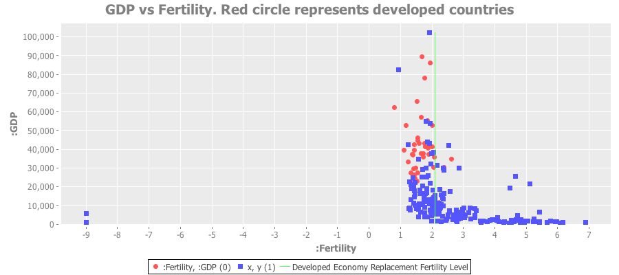
Singapore’s government (and Mentos was involved in this awkward project) used this ad on their National Day celebrations to encourage people to copulate and increase Singapore’s birth rate. I hypothesized that a low fertility rate (number of children per woman) was not unique to Singapore (though the problem might be more acute in Singapore).

Here’s a plot of GDP vs. fertility rates for all nations. The red dots are the devloped countries:

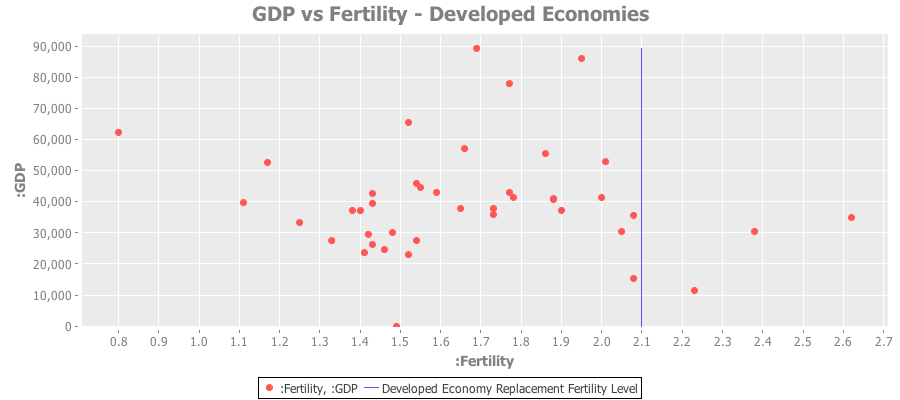
Clearly the poorest nations have a ridiculously high fertility rate. The red dots represent the developed economies - almost all of which lie below the replacement fertility rate of 2.1

Here’s a plot of just the developed economies:

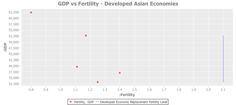
And a similar plot for developed Asian economies:

Full source code and datasets available in this github repo.